The Silent Architect: How PostgreSQL Statistics Shape Your Query Performance
In the complex ecosystem of relational database management systems, PostgreSQL stands out for its sophisticated query planner—a component often mistaken for a black box. Behind every SELECT statement lies a series of high-stakes calculations performed by the query planner, which determines the most efficient path to retrieve your data. However, the planner does not possess clairvoyance; it operates based on a curated, statistical summary of your database known as pg_stats.
As discussed at POSETTE 2026, understanding the relationship between these statistics and the query planner is the difference between a high-performance application and one plagued by inexplicable latency. When developers encounter slow queries, the knee-jerk reaction is often to blame the database engine or the hardware. In reality, the culprit is frequently a disconnect between the database’s "mental model" of the data and the actual distribution of that data.
The Architecture of Decision-Making
When a SQL query is submitted to PostgreSQL, it is parsed and rewritten, eventually arriving at the query planner. The planner’s goal is to minimize the "cost" of the query. Crucially, the planner does not perform a live scan of the entire dataset to determine this cost, as doing so would be prohibitively expensive for large tables. Instead, it relies on pg_statistic, a system catalog that stores metadata about the contents of your tables.
For human readability, PostgreSQL exposes this data through the pg_stats view. This view provides a window into the planner’s assumptions, covering metrics such as the number of distinct values in a column, the fraction of null values, and the physical correlation between the data’s order on disk and its logical order.
Chronology of a Query Plan
The lifecycle of a query plan begins with the ANALYZE command. Without this command, the planner would be operating in the dark.
- Data Sampling: When
ANALYZEruns—either manually or automatically via the autovacuum process—it scans a statistical sample of the table. - Summary Construction: It calculates column-specific metrics, identifying data density and distribution.
- Storage: These metrics are written to the
pg_statisticsystem catalog. - Planning: When a user executes a query, the planner consults these statistics to estimate the number of rows (cardinality) that will be returned by a specific filter.
- Execution Strategy: Based on those estimates, the planner chooses between a sequential scan (reading the entire table) or an index scan (jumping directly to specific rows).
The tension arises when the data changes rapidly. If a table undergoes massive inserts or deletions and ANALYZE hasn’t caught up, the statistics become stale. An outdated summary leads to a "guess" that is fundamentally wrong, resulting in the planner choosing an inefficient execution path.
Supporting Data: The Case of the "CA" Query
To illustrate this, consider a customers table with one million rows. If you query for WHERE state = 'CA', you might expect the database to use an index on the state column. However, if the planner sees that ‘CA’ appears in 17% of your rows, it may correctly determine that a sequential scan is faster than performing 170,000 individual index lookups.
The decision is based on cost parameters:
- seq_page_cost: The cost of fetching a page sequentially.
- random_page_cost: The cost of a non-sequential disk fetch.
- cpu_tuple_cost: The cost of processing an individual row.
When the query planner estimates the cost of a plan, it calculates these values against the cardinality estimate. If the estimate for ‘CA’ is off, the planner might choose an index scan when a sequence scan would have been faster, or vice versa, leading to massive performance regressions.
The Role of Most Common Values (MCV)
One of the most powerful tools in the planner’s arsenal is the Most Common Values (MCV) list. ANALYZE keeps a list of the most frequent values in a column and their specific frequencies. This allows the planner to handle skewed data distributions gracefully.
In the example of our customers table, the MCV list identifies that ‘CA’ occurs 17.4% of the time, while ‘WY’ might occur only 0.4% of the time. Because the planner knows the exact frequency of ‘WY’, it can accurately estimate that an index scan is the most efficient path for that specific search. This granular understanding is what prevents "plan flip-flopping" where queries work perfectly for some parameters but fail catastrophically for others.
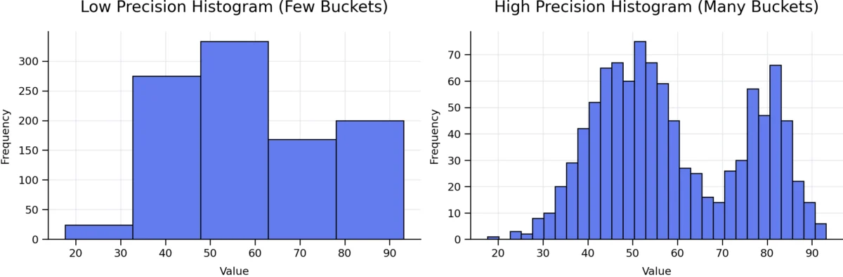
Histograms and Precision
While MCVs handle equality, histograms handle range-based queries (e.g., signup_date BETWEEN '2025-01-01' AND '2025-03-01'). By default, PostgreSQL creates a 100-bucket equi-depth histogram for each column.
If your data is highly skewed—for instance, if 90% of your signups happened in a single month—a standard 100-bucket histogram might lack the resolution to distinguish between specific days within that month. Developers can address this by adjusting the STATISTICS target for specific columns:
ALTER TABLE customers ALTER COLUMN signup_date SET STATISTICS 1000;
ANALYZE customers;
By increasing the number of buckets, you provide the planner with a higher-resolution map of the data. However, this is a double-edged sword: larger histograms require more memory for the statistics object and increase the time spent during the planning phase. It is a classic engineering trade-off: precision for the query planner versus overhead for the system.
Implications of Correlated Data
Perhaps the most significant challenge in query planning is the assumption of column independence. By default, the planner assumes that if you filter by city = 'Cheyenne' and state = 'WY', the probability of both being true is the product of their individual probabilities.
In reality, these columns are highly correlated. This leads to severe under-estimation of row counts, often by several orders of magnitude. When the planner underestimates the number of rows, it may choose an nested-loop join when a hash join would have been far more efficient.
Since PostgreSQL 10, developers can use CREATE STATISTICS to inform the planner of these relationships:
CREATE STATISTICS customers_city_state (dependencies, ndistinct)
ON city, state FROM customers;
This simple command creates a multi-column statistics object that forces the planner to recognize that filtering by ‘Cheyenne’ inherently filters by ‘WY’. The resulting plan is not only more accurate in its row estimates but also significantly more performant in its execution.
The Developer’s Checklist for Performance
When faced with a query that defies logic, follow this systematic approach:
- Check for Stale Statistics: Does
pg_statsreflect the current state of the data? RunANALYZEmanually if needed. - Verify Row Estimates: Use
EXPLAIN ANALYZEto compare the "estimated rows" versus "actual rows." A massive discrepancy is a smoking gun. - Inspect MCVs: Does your query involve a value in the MCV list? If not, the planner might be using a less-accurate default estimate.
- Evaluate Histogram Precision: Are you dealing with complex range queries on skewed data? Consider increasing the
STATISTICStarget. - Identify Correlations: Are you filtering on multiple columns that share a logical relationship? Use extended statistics.
- Avoid "Quick Fix" Anti-patterns: Avoid disabling
seqscanorindexscanglobally. These settings act as blunt instruments that can break other parts of your application.
Conclusion
The PostgreSQL query planner is an engineering marvel, but it is bound by the quality of the information it receives. It is not an omniscient entity; it is a statistical processor. When performance suffers, the problem is rarely that the planner is "broken"—it is almost always that the planner is "misinformed."
By mastering pg_stats, developers move from the role of reactive troubleshooters to proactive architects. Understanding how to guide the planner—through manual analysis, target adjustments, and extended statistics—is a hallmark of a senior database engineer. As the saying goes, the query planner is only as smart as the statistics you feed it. Treat those statistics with the same care you treat your code, and your database will reward you with consistent, predictable, and high-speed performance.