Revolutionizing Time-Series Engineering: How Google and Tryolabs Simplify Temporal Machine Learning with Temporian and TensorFlow Decision Forests

MOUNTAIN VIEW, Calif. — In the rapidly evolving landscape of applied machine learning, the ability to effectively process, model, and extract signal from time-varying information remains one of the industry’s most persistent bottlenecks. Whether it is financial transactions fluctuating by the second, network logs flagging sudden intrusion attempts, or biometric data measuring the subtle intervals between heartbeats, temporal data is ubiquitous. Yet, preparing this data for machine learning models has historically required complex, bespoke codebases prone to data leakage, scalability issues, and painful joins across non-synchronized sources.

To address this challenge, a collaborative engineering effort between Google and AI solutions provider Tryolabs has yielded Temporian—a powerful open-source Python library designed specifically to streamline the preprocessing and feature engineering of temporal data. Combined with the robustness of TensorFlow Decision Forests (TFDF), data scientists and machine learning engineers now possess a streamlined, end-to-end pipeline to ingest raw event streams, compute sophisticated rolling metrics, and train production-grade forecasting and classification models with unprecedented ease.

Main Facts: The Intersection of Temporian and TensorFlow Decision Forests

At its core, temporal data presents unique structural challenges that traditional tabular frameworks struggle to accommodate. Standard machine learning workflows often assume static, independent observations. However, real-world applications rely heavily on history, context, and the temporal relationships between events.

Pre-processing temporal data made easier with TensorFlow Decision Forests and Temporian

Temporian introduces a generalized container for temporal data known as the EventSet. Unlike classical time series—which rely on uniformly sampled values—EventSets support multivariate, multi-index time sequences capable of ingesting non-uniformly sampled measurements and complex relational data.

When paired with TensorFlow Decision Forests, particularly Random Forest regression architectures, Temporian bridges the gap between raw transactional logs and structured, tabular machine learning datasets. The synergy allows practitioners to:

Ingest raw, multi-source event data natively without manual resampling loops.
Compute complex temporal aggregations (such as moving sums, moving averages, and calendar features) across different categorical indexes effortlessly.
Convert processed temporal data directly into TensorFlow-compatible datasets for rapid model training and evaluation.
Analyze feature importances to determine precisely which temporal horizons drive predictive accuracy.

Chronology: The Evolution of Temporal Data Preparation

For years, the engineering lifecycle for temporal machine learning projects followed a grueling trajectory. Understanding how Temporian alters this paradigm requires examining the historical evolution of how developers handled time-dependent data.

Phase 1: The Era of Manual Pandas Resampling

In the early days of applied data science, engineers relied heavily on Python libraries like Pandas. While exceptional for in-memory data manipulation, Pandas was never architected for high-performance temporal feature engineering at scale. Calculating rolling windows across millions of non-synchronized client transactions required writing custom grouping loops, handling missing timestamps manually, and risking devastating target leakage—a phenomenon where future information inadvertently taints the training features.

Phase 2: Specialized Streaming and Windowing Frameworks

As big data architectures matured, frameworks like Apache Beam and Apache Spark introduced distributed data processing. While these tools solved scale, they imposed a heavy infrastructure tax. Data scientists had to master distributed stream-processing paradigms just to compute a 30-day moving average on user purchase history, dragging down development velocity.

Phase 3: The Birth of Temporian

Recognizing the desperate need for a dedicated, pythonic, and high-performance solution, engineers at Google and Tryolabs banded together to build Temporian. Released as an open-source library, Temporian was engineered from the ground up to treat time as a first-class citizen. It abstracts away the complexities of continuous-time indexing, allowing developers to write concise, readable code that mirrors mathematical definitions of temporal operators.

Supporting Data: A Practical Walkthrough of Sales Forecasting

To understand the practical mechanics of this stack, consider a canonical machine learning use case: forecasting weekly and daily sales from a raw transactional log generated by an online storefront.

1. Ingesting and Visualizing Raw Transactions

A typical dataset arrives as a CSV file containing individual transaction records, complete with precise timestamps, client identifiers, product codes, and purchase prices:

timestamp,client,product,price
2010-10-05 11:09:56,c64,p35,405.35
2010-09-27 15:00:49,c87,p29,605.35
2010-09-09 12:58:33,c97,p10,108.99
2010-09-06 12:43:45,c60,p85,443.35

Using Temporian, loading this data into an EventSet requires just a few lines of Python:

import temporian as tp

# Load the csv dataset into a Temporian EventSet
sales = tp.from_csv("/tmp/sales.csv")

# Plot the raw price feature
sales["price"].plot()

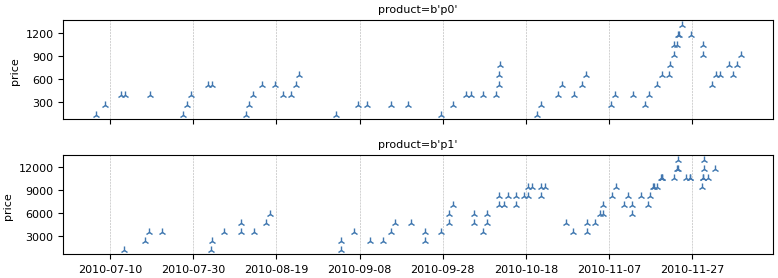
Because raw transaction logs contain spikes and dips across multiple distinct clients and products simultaneously, the resulting visualization is often dense and noisy. To extract meaningful signals, engineers apply windowing operators, such as calculating a moving sum over a trailing seven-day window:

# Compute the 7-day moving sum of sales
weekly_sales = sales["price"].moving_sum(tp.duration.days(7))
weekly_sales.plot()

2. Indexing and Granular Aggregations

In real-world business scenarios, global store metrics are rarely sufficient; organizations require granular insights per product or per customer. Temporian handles this via native indexing capabilities:

# Index the data by product category
sales_per_product = sales.add_index("product")

# Compute the moving sum independently for each product
weekly_sales_per_product = sales_per_product["price"].moving_sum(
    tp.duration.days(7)
)
weekly_sales_per_product.plot()

Furthermore, practitioners can sample this continuous transactional data into uniform daily intervals using the tick operator, preparing it for tabular machine learning models:

# Sample the data daily
daily_sampling = sales_per_product.tick(tp.duration.days(1))

# Calculate daily aggregates with a trailing weekly window
weekly_sales_daily = sales_per_product["price"].moving_sum(
    tp.duration.days(7),
    sampling=daily_sampling
)

3. Dataset Augmentation and Machine Learning Integration

With feature engineering complete, the next step involves generating multi-horizon features and shifting target variables to build a supervised learning dataset. By computing moving sums across various window lengths (e.g., 3, 7, 14, and 28 days) alongside calendar features like the day of the week, models gain a rich contextual understanding of human buying patterns.

features = []
for w in [3, 7, 14, 28]:
    features.append(
        sales_per_product["price"]
        .moving_sum(tp.duration.days(w), sampling=daily_sampling)
        .rename(f"moving_sum_w")
    )

# Add calendar features
features.append(daily_sampling.calendar_day_of_week())

# Define the label: next day's sales (using temporal leakage prevention)
label = (
    sales_per_product["price"]
    .leak(tp.duration.days(1))
    .moving_sum(tp.duration.days(1), sampling=daily_sampling)
    .rename("label")
)

# Combine features and labels into a unified Temporian dataset
dataset = tp.glue(*features, label)

Finally, this dataset transitions seamlessly into TensorFlow format to train a Random Forest regression model via TensorFlow Decision Forests:

import tensorflow_decision_forests as tfdf

def extract_label(example):
    example.pop("timestamp") # Exclude raw timestamps as features
    label = example.pop("label")
    return example, label

tf_dataset = tp.to_tensorflow_dataset(dataset).map(extract_label).batch(100)

# Train a Random Forest Regression model
model = tfdf.keras.RandomForestModel(task=tfdf.keras.Task.REGRESSION, verbose=2)
model.fit(tf_dataset)

Official Responses: Perspectives from the Development Teams

The release of Temporian represents a strategic alignment between tech giants and specialized engineering boutiques to solve foundational data science pain points.

Mathieu Guillame-Bert, speaking on behalf of the Google development team, emphasized the philosophical shift behind the library: "Temporal data is the lifeblood of modern enterprise intelligence. However, the friction involved in cleaning, aligning, and engineering features from time-series data has historically slowed down innovation. By combining Temporian’s intuitive time-first abstractions with TensorFlow Decision Forests, we are empowering developers to focus on model architecture and business logic rather than writing brittle preprocessing plumbing."

Partners at Tryolabs echoed these sentiments, highlighting the cross-domain adaptability of the library. From fraud detection in financial systems to predictive maintenance in industrial Internet of Things (IoT) deployments, the ability to process asynchronous event streams cleanly has immediate commercial value. Tryolabs engineers noted that the library’s design prevents common pitfalls such as data leakage, ensuring that models trained in development environments maintain robust performance when deployed to production streaming pipelines.

Implications: What This Means for the Future of Applied AI

The integration of Temporian and TensorFlow Decision Forests carries profound implications for the broader machine learning engineering community.

1. Democratization of Advanced Time-Series Modeling

Historically, building robust time-series forecasting models required deep expertise in specialized statistical packages or complex stream-processing frameworks. By abstracting these complexities into clean Pythonic primitives, Temporian lowers the barrier to entry. Junior and senior data scientists alike can construct complex, multi-indexed rolling features with minimal code, accelerating the prototyping and deployment lifecycle.

2. Enhanced Model Interpretability

As demonstrated through TensorFlow Decision Forests’ variable importance metrics (such as INV_MEAN_MIN_DEPTH), models trained on Temporian-preprocessed data offer deep transparency. In our sales forecasting example, model summaries revealed that the 28-day moving sum (moving_sum_28) held the highest predictive importance (0.342), closely followed by product categorization and calendar day-of-week attributes. This level of explainability is vital for enterprise stakeholders who require audited, understandable decision-making systems.

3. Bridging Tabular and Temporal Domains

While deep learning architectures like LSTMs and Transformers have dominated time-series discourse, gradient-boosted decision trees (GBDTs)—via TensorFlow Decision Forests—remain the gold standard for tabular and semi-structured business data due to their speed, resilience to overfitting, and ease of tuning. Temporian successfully bridges these worlds, allowing GBDT architectures to ingest rich, continuous temporal streams without forcing engineers to abandon tabular workflows.

Next Steps for Practitioners

For developers and data scientists eager to modernize their time-series pipelines, the open-source repositories and documentation are fully accessible:

Explore the official Temporian Documentation and Tutorials for domain-specific examples spanning finance, retail, and IoT.
Dive into TensorFlow Decision Forests to learn more about training high-performance gradient-boosted trees and random forests.
Review the foundational design philosophy via the Tryolabs and Google Introduction Post.

As temporal data continues to scale in volume and complexity, tools like Temporian and TensorFlow Decision Forests ensure that engineering teams remain equipped to turn raw event streams into actionable, predictive intelligence.